Back to NEISS – NLP and Classification

In my last post, I performed some exploratory analysis on the NEISS dataset, which is a sample of hospital visits in the US that are related to consumer products. I wanted to return to this dataset and work on some predictive modeling. In particular, I will be trying to predict the location where an injury happened. As will be seen later, a simple model actually works surprisingly well for this task. However, this post is mostly an excuse for me to work on some NLP techniques.

Let’s load up the data again and get started!

neiss = pd.read_csv('neiss.csv')
print(neiss.shape)
print(neiss.columns)

## (1841588, 27)

## Index(['CPSC_Case_Number', 'Treatment_Date', 'Year', 'Age', 'Sex', 'Race',
##       'Other_Race', 'Hispanic', 'Body_Part', 'Diagnosis', 'Other_Diagnosis',
##       'Body_Part_2', 'Diagnosis_2', 'Other_Diagnosis_2', 'Disposition',
##       'Location', 'Fire_Involvement', 'Alcohol', 'Drug', 'Narrative',
##       'Stratum', 'PSU', 'Weight', 'Product', 'Product_2', 'Product_3'],
##      dtype='object')

This is a pretty large dataset, and the different columns provide a good glimpse on how injuries occurred. However, for this project, I will only be focusing on two columns: Location and Narrative.

neiss['Location'].value_counts(normalize=True)

## Home                             0.439636
## Not recorded                     0.283534
## Place of recreation or sports    0.130473
## Other public property            0.070278
## School/Daycare                   0.053731
## Street or highway                0.021715
## Farm/ranch                       0.000347
## Mobile/Manufactured home         0.000212
## Industrial                       0.000074

As can probably be inferred, the Location column indicates where an injury took place. Unfortunately, the location has a value of “Not recorded” for over a quarter of the observations in the dataset. This inspired me to try to find a way to predict the location of the injury for these observation where it is not recorded. To accomplish this, I made use of the Narrative column, which gives a short description of how an injury occurred.

neiss['Narrative'].head(3)

Narrative
14 YOM SUSTAINED A CLOSED HEAD INJURY AFTER PASSING OUT AND HITTING HIS HEAD ON SOME STEPS
32YOM WAS CAST FISHING IN THE BAY WHEN HE CAME OUT HE HAD A RASH TO LOWER LEGS CONTACT DERMATITIS
43YOF STR LWR BACK - MOVING FURNITURE

The basic idea is that certain words within these descriptions will give a good indication of where the injury took place. Thus, by utilzing some NLP techniques, I should be able to create a good predictor of an injury’s location.

Before any model building, I need to pre-process the data. This means creating a new columns called Text, which is a cleaned up version of the Narrative column. First, I removed the rows which have a value of “Not recorded” since these are essentially unlabeled data points. I also removed rows with the values of “Farm/ranch”, “Mobile/Manufactured home”, and “Industrial” in Location since these are quite rare. Next, I wanted to change the data type in the Location column from string data into numerical data with a Label Encoder. Then, I had to clean the string data in the Narrative column to help remove irrelevant noise. This involves things like removing characters that are not alphanumeric, making all the strings lower case, and fixing some differences in medical abbreviations. Finally, I tokenized the data. This means that for each string in the Text column, I broke the string down into a list of individual words. This is accomplished with the Natural Language Toolkit, or nltk.

from sklearn.preprocessing import LabelEncoder
from nltk.tokenize import RegexpTokenizer

neiss_clf = neiss[['Location', 'Narrative']]
neiss_clf = neiss_clf.loc[~neiss['Location'].isin(['Not recorded', 'Farm/ranch',
                             'Mobile/Manufactured home', 'Industrial']) == True]

le = LabelEncoder()
le.fit(list(neiss_clf['Location'].unique()))
neiss_clf['Location_label'] = le.transform(neiss_clf['Location'])

neiss_clf['Text'] = neiss_clf['Narrative'].str.replace(r'[^a-zA-Z0-9 ]+', ' ')
    .str.lower().str.replace('yof', ' yof ')
    .str.replace('yom', ' yom ').str.replace('yf', ' yof ')
	.str.replace('ym', ' yom ').str.replace('yo f', ' yof ')
	.str.replace('yo m', ' yom ').str.replace('yr', ' yr ')
	.str.replace('dx', ' dx ').str.replace('tx', ' tx ')
	.str.replace('hx', ' hx ')

tokenizer = RegexpTokenizer(r'\w+')
neiss_cld["Tokens"] = neiss_clf["Text"].apply(tokenizer.tokenize)

neiss_clf.head()

Location	Narrative	Location_label	Text	Tokens
Home	21 DAY OLD FEMALE WAS IN BED WITH MOM, WHEN MOM WOKE UP SHE NOTICEDBABY WASN’T BREATHING, DRIED BLOOD ON NOSE. DX: CARDIAC ARREST	0	21 day old female was in bed with mom when mom woke up she noticedbaby wasn t breathing dried blood on nose dx cardiac arrest	[‘21’, ‘day’, ‘old’, ‘female’, ‘was’, ‘in’, ‘bed’, ‘with’, ‘mom’, ‘when’, ‘mom’, ‘woke’, ‘up’, ‘she’, ‘noticedbaby’, ‘wasn’, ‘t’, ‘breathing’, ‘dried’, ‘blood’, ‘on’, ‘nose’, ‘dx’, ‘cardiac’, ‘arrest’]
Place of recreation or sports	11 YOM ICE SKATING FELL BACKWARDS HIT HEAD DX CONCUSSION	2	11 yom ice skating fell backwards hit head dx concussion	[‘11’, ‘yom’, ‘ice’, ‘skating’, ‘fell’, ‘backwards’, ‘hit’, ‘head’, ‘dx’, ‘concussion’]
Home	54YOF WAS IN THE SHOWER SLIPPED FELL BACKWARDS HITTING HEAD W/ BLURRY VISION AFTER DX HEAD INJ	0	54 yof was in the shower slipped fell backwards hitting head w blurry vision after dx head inj	[‘54’, ‘yof’, ‘was’, ‘in’, ‘the’, ‘shower’, ‘slipped’, ‘fell’, ‘backwards’, ‘hitting’, ‘head’, ‘w’, ‘blurry’, ‘vision’, ‘after’, ‘dx’, ‘head’, ‘inj’]

There’s just one more thing that needs to be done before I can create my first predictor. I need a way to represent these word tokens numerically so that they can be used for modeling. To start, I used a simple way to achieve this: a bag-of-words model. What this model does is first create a vocabulary list of all unique words in the Text column. Then, it represents each string as a vector which counts how many times a word appears. This is considered a simple method because it only considers word count and ignores contextual information like word order.

Also, I took a sample of 500,000 random observations from the dataset. This is to save on computation time when fitting models.

from sklearn.feature_extraction.text import CountVectorizer
from sklearn.model_selection import train_test_split

sample = neiss_clf.sample(300000)
from sklearn.feature_extraction.text import CountVectorizer
from sklearn.model_selection import train_test_split

list_corpus = sample['Text'].tolist()
list_labels = sample['Location_label'].tolist()

X_train_val, X_test, y_train_val, y_test = train_test_split(list_corpus, list_labels, random_state=42,
                                                            test_size=0.2)
X_train, X_val, y_train, y_val = train_test_split(X_train_val, y_train_val, random_state=42,
                                                  test_size=0.2)

count_vect = CountVectorizer()
X_train_counts = count_vect.fit_transform(X_train)
X_val_counts = count_vect.transform(X_val)

Now that the data is ready, it is time to create a basic model to predict the location of injuries. I started with a linear SVM since this is often one of the best classifiers for text. I left all the hyperparamters at their default values.

from sklearn.feature_extraction.text import CountVectorizer
from sklearn.model_selection import train_test_split
from sklearn.metrics import accuracy_score, f1_score, precision_score, recall_score
from sklearn.linear_model import SGDClassifier
from sklearn.pipeline import Pipeline
    

def bow(token, data=sample):
    text = token.apply(lambda x: ' '.join(x))
    list_corpus = text.tolist()
    list_labels = data['Location_label'].tolist()
    X_train_val, X_test, y_train_val, y_test = train_test_split(list_corpus, list_labels,
                                                            test_size=0.2)

    X_train, X_val, y_train, y_val = train_test_split(X_train_val, y_train_val,
                                                  test_size=0.2)
    count_vect = CountVectorizer()

    X_train_counts = count_vect.fit_transform(X_train)
    X_val_counts = count_vect.transform(X_val)
    return X_train, X_val, y_train, y_val, X_test, y_test, X_train_counts, X_val_counts

X_train, X_val, y_train, y_val, X_test, y_test, X_train_counts, X_val_counts = bow(sample['Tokens'])

clf = SGDClassifier()
clf.fit(X_train_counts, y_train)
y_pred = clf.predict(X_val_counts)

def get_metrics(y_test, y_pred):  
    precision = precision_score(y_test, y_pred, pos_label=None,
                                    average='weighted')             
    recall = recall_score(y_test, y_pred, pos_label=None,
                              average='weighted')
    f1 = f1_score(y_test, y_pred, pos_label=None, average='weighted')
    accuracy = accuracy_score(y_test, y_pred)
    return accuracy, precision, recall, f1

accuracy, precision, recall, f1 = get_metrics(y_val, y_pred)
print("accuracy = %.3f, precision = %.3f, recall = %.3f, f1 = %.3f" % (accuracy, precision, recall, f1))
	
## accuracy = 0.902, precision = 0.905, recall = 0.902, f1 = 0.897

Wow! This simple model was able to achieve around 90% in accuracy, precision, recall, and f1. Let’s try to visualize the bag-of-word vectors in order to see how the model is able to achieve such surprisingly well-performing results. With over 50,000 unique words in the vocabulary list, each vector has over 50,000 dimensions. However, we can use perform dimensionality-reduction to project the data down to two dimensions and create a plot.

from sklearn.decomposition import TruncatedSVD
import matplotlib.pyplot as plt
import seaborn as sns
import matplotlib.patches as mpatches

truncate = TruncatedSVD(n_components=2)
truncated_x = truncate.fit_transform(X_train_counts)

sns.set(font_scale = 1.5)
a4_dims = (11.7, 8.27)
fig = plt.subplots(figsize=a4_dims)
colors = {0:'royalblue', 1:'darkgreen', 2:'orange', 3:'darkviolet', 4:'red'}
ax = sns.scatterplot(x=truncated_x[:, 0], y=truncated_x[:, 1], hue=y_train, palette=colors, s=25)
dot1 = mpatches.Patch(color='royalblue', label='Home')
dot2 = mpatches.Patch(color='darkgreen', label='Other Public Property')
dot3 = mpatches.Patch(color='orange', label='Place of Recreation/Sport')
dot4 = mpatches.Patch(color='darkviolet', label='School/Daycare')
dot5 = mpatches.Patch(color='red', label='Street')
ax.legend(handles=[dot1, dot2, dot3, dot4, dot5])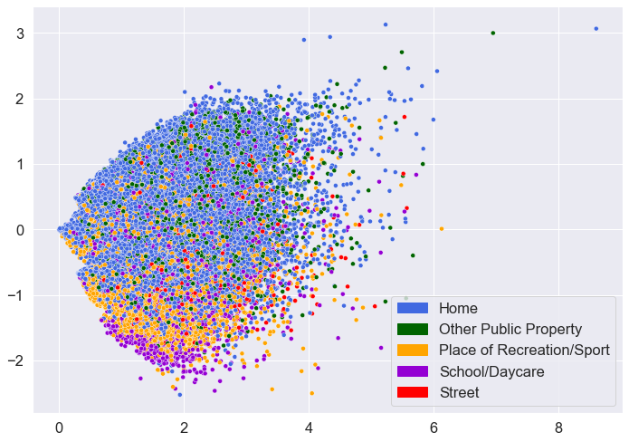

While there is definitely overlap among the different locations, there also appears to be some patterns. In particular, the data points for “Home”, “Place of Recreation/Sport”, and “Street” seem to be clustering together somewhat.

Another way to gain insights on one’s model is to create a confusion matrix. A confusion matrix is a good way to show how exactly your model is making mistakes in classification.

from sklearn.metrics import confusion_matrix

cm = confusion_matrix(y_val, y_pred)
labels = ['Home', 'Other Public Property', 'Place of Recreation/Sport', 'School/Daycare',
          'Street']
df_cm = pd.DataFrame(cm, index = [i for i in labels],
                  columns = [i for i in labels])

ax = sns.heatmap(df_cm, annot=True, cmap="YlGnBu", fmt='g')
ax.set_ylabel('True Label', weight='bold', labelpad=15)
ax.set_xlabel('Predicted Label', weight='bold', labelpad=15)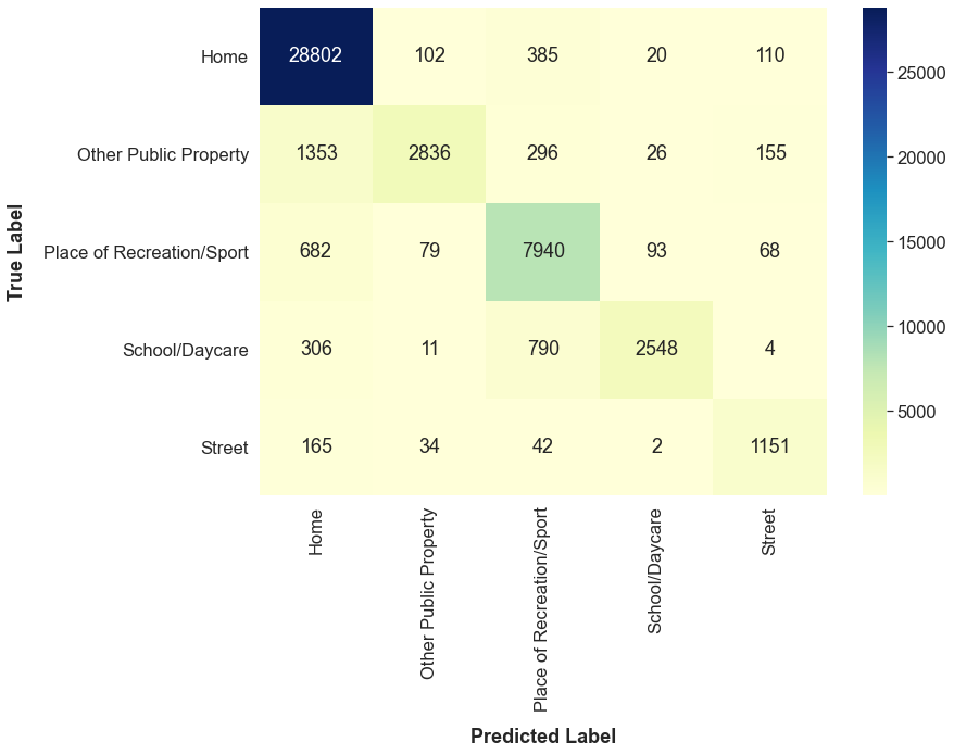

At a quick glance, I can see that the model frequently predicts “Home” for data points that have the true label of “Other Public Property.” Actually, this result could have been anticipated. When looking at the scatterplot above, there does not seem to be any differences in the locations of the blue points and the green points.

Now that I have my base model, it’s time to make improvements. While the base model performed well, I want to see if I can make it even better. First, I tried to accomplish this by filtering out stop words. Stop words refer to the most common words in a language. For English, these are words like “the”, “is”, “at”, “on”, etc. The idea is that these words occur so often that they provide basically no information that can help with classification. By removing them, you are making your dataset smaller which decreases the time to train your model. Also, after removing them, you are only left with more significant words, so your model’s performance may increase. I removed the stop words generated by Text and re-trained my model.

nltk.download('stopwords')
from nltk.corpus import stopwords
stopword = set(stopwords.words('english'))

def remove_stop(tokens):
    text = [word for word in tokens if word not in stopword]
    return text

sample['Tokens_nostop'] = sample['Tokens'].apply(lambda x: remove_stop(x))

X_train, X_val, y_train, y_val, X_test, y_test, X_train_counts, X_val_counts = bow(sample['Tokens_nostop'])

clf = SGDClassifier()
clf.fit(X_train_counts, y_train)
y_pred = clf.predict(X_val_counts)
accuracy, precision, recall, f1 = get_metrics(y_val, y_pred)
print("accuracy = %.3f, precision = %.3f, recall = %.3f, f1 = %.3f" % (accuracy, precision, recall, f1))
## accuracy = 0.899, precision = 0.903, recall = 0.899, f1 = 0.894

After removing the stop words, the model’s predictions actually got worse. In some way, the stop words were helping my model make better predictions so I decided to keep the stop words and not remove them.

Another common pre-processing technique for text data is to lemmatize the data. Lemmatization is a term referring to grouping together words that have the same root. For example, words like “fallen” or “fell” would be transformed into the root word “fall.”

To be continued! Concepts to add: stop words, lemmatization, TF-IDF, BERT, and model selection

Stuart Wilson